[PAPER REVIEW] QTran: Learning to Factorize with Transformation

As explained by Kasim Te and Yajie Zhou.

I recently read QTRAN: Learning to Factorize with Transformation for Cooperative Multi-Agent Reinforcement Learning [1], and also met with the primary author to discuss its details. Here are some of my notes.

1. What is QTran?
2. What is the factorization approach?
3. Motivation: Previous Approaches
4. What about this game, though?
5. What is QTran’s approach?
6. What does the architecture look like?
7. How does this even work?
8. More
9. References

What is QTran?

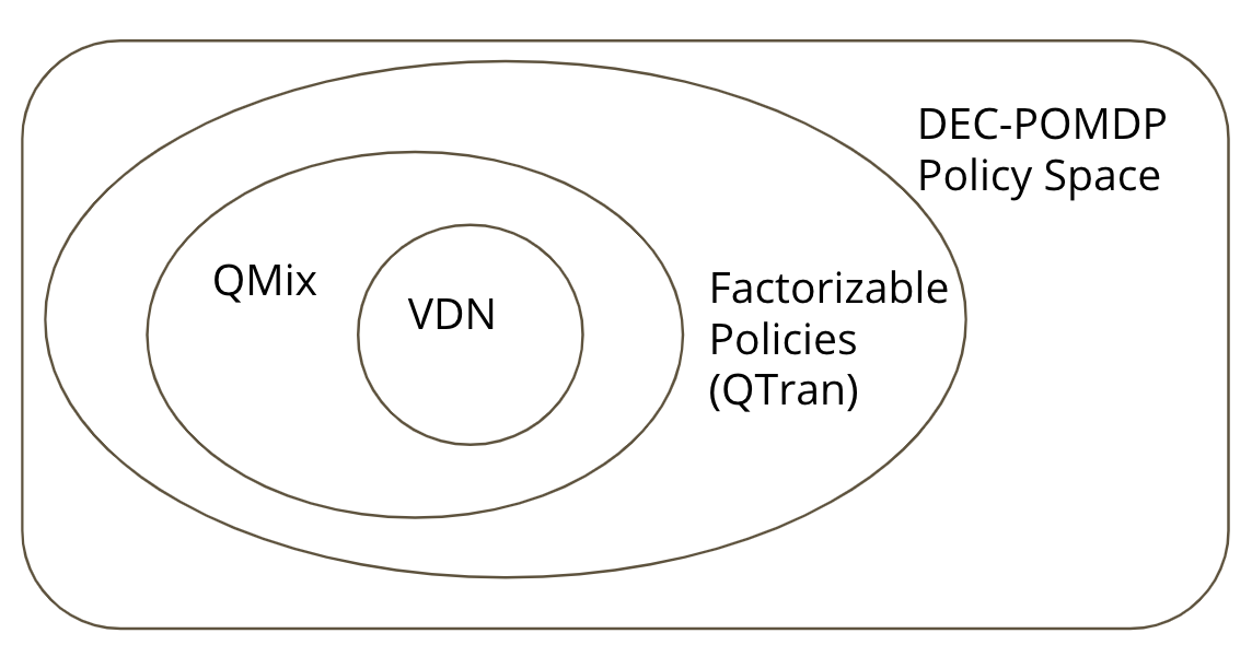
QTran is a value-based solution to a multi-agent reinforcement learning (MARL) task, focusing on centralized training and decentralized execution (CTDE). Although the global state may be used during training, at execution time, each agent uses an individual policy to determine actions, which is based on that agent’s observation (often partial) of the global state. This type of task is referred to as a decentralized partially observable markov decision process (DEC-POMDP).

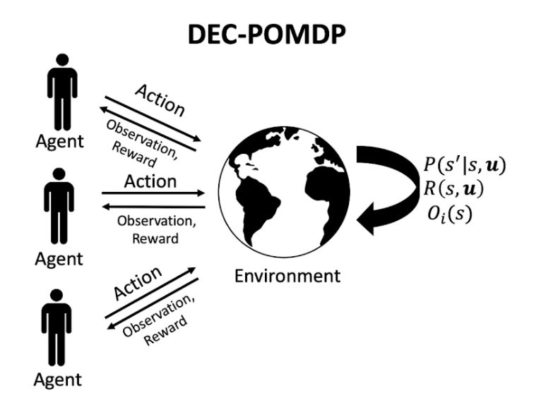
Here,

• P is the probability of the next state s’ based on the current state s and joint action u.
• R is the shared reward function based on the current state s and joint action u.
• O is the observation function for agent i based on the current state s.

The setting is cooperative, so agents share the reward.

What is the factorization approach?

QTran takes a factorization approach, in which the optimal joint action-value Q function (on which the optimal joint policy is based) is decomposed into individual Q functions for each agent to determine decentralized individual policies for each agent.

A joint Q function is said to be factorizable into individual agent Q functions if the following holds:

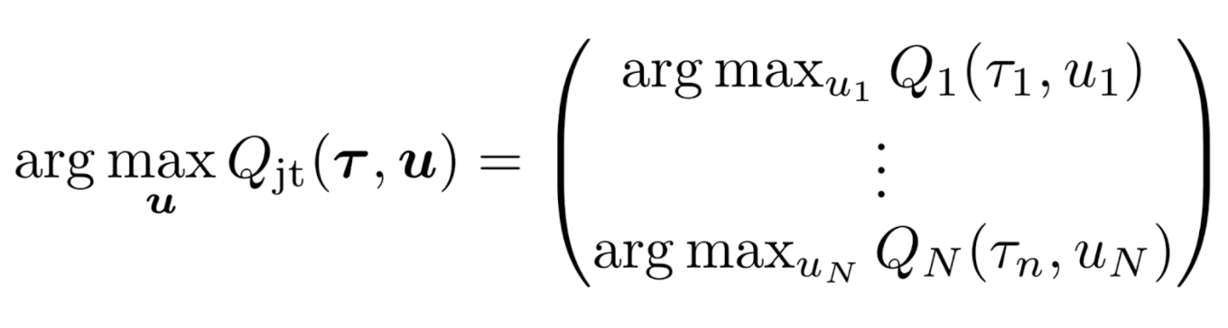
In the above, u is the joint action and tau is the state, represented as the joint action-observation history. If the optimal joint action is equivalent to the set of optimal individual actions [u-i], then the joint Q function is said to be factorizable by the individual Q functions. In such a scenario, executing the optimal individual policies based on the individual Q functions will result in optimizing the joint Q function as well, even if executing in a decentralized manner.

Motivation: Previous Approaches

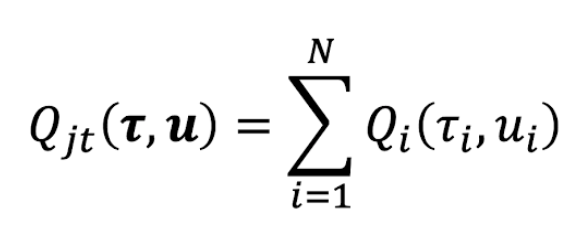
VDN and QMix [2] are two prior representative factorization approaches. They learn a joint Q function and ensure factorizability by adding a sufficient condition as a constraint. More specifically, VDN ensures it via additivity:

And QMix, via monotonicity:

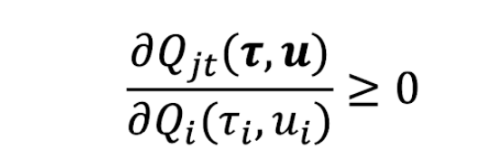
In the first, as the joint Q is simply the sum of the individual Q functions, maximizing any individual Q function will also maximize the joint Q function. The second expands upon this and allows non-linear relationships between the joint Q and each individual Q, as long as monotonicity is preserved.

What about this game, though?

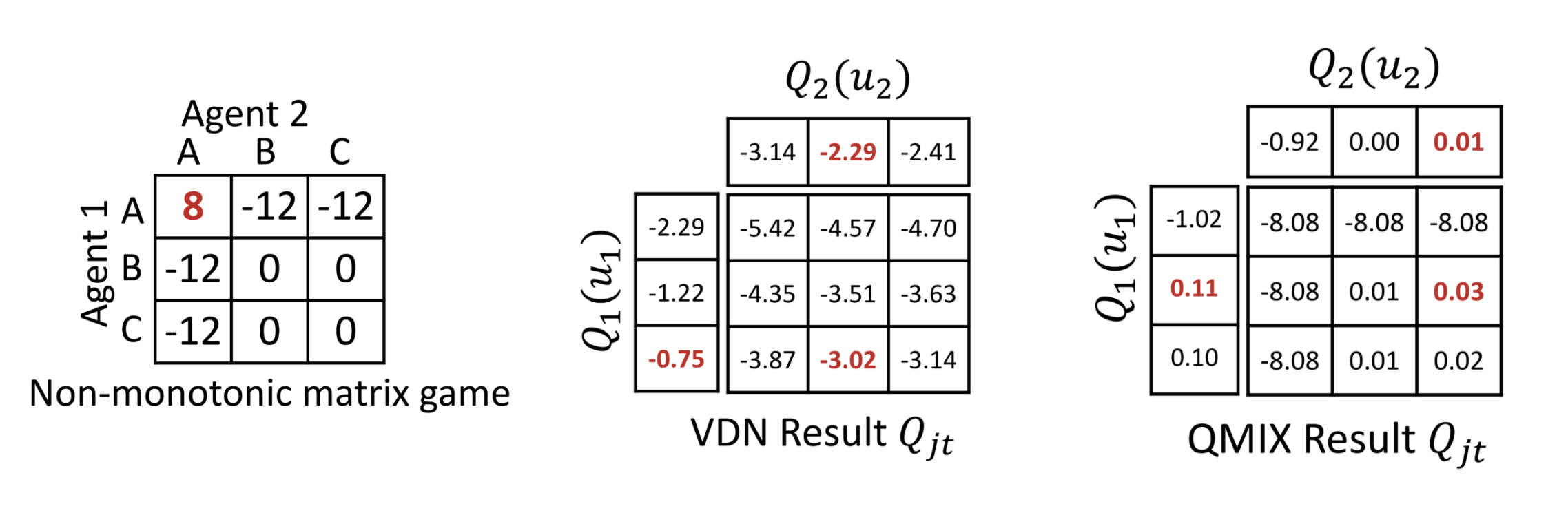
What’s the optimal joint action of the non-monotonic matrix game on the left? It doesn’t take long to see it is for both players to choose A. And yet VDN and QMIX both fail to learn the optimal joint action.

In many scenarios, the true joint Q function is likely very complex. It is possibly not convex and possibly not monotonic. In fact, it is possibly not even factorizable. And since the learned joint Q function from VDN and QMix are bound by the above constraints, they cannot express dynamics that are not additive or monotonic, respectively.

What is QTran’s approach?

QTran’s approach loosens the constraints and learns a joint Q function with any possible factorization.

It does so by specifying the following constraint:

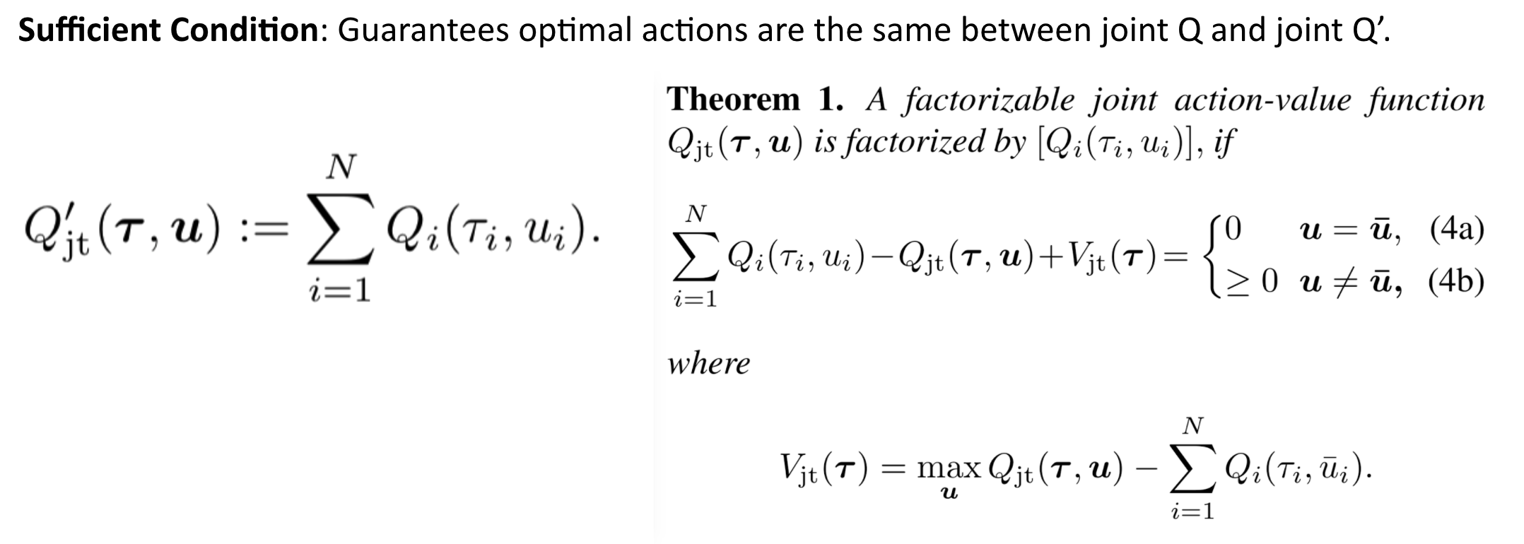
How does this work? QTran learns a joint Q function and uses a separate, transformed joint Q prime function to ensure factorization, where the transformed joint Q prime function is defined as the sum of the individual Q functions. The objective loss function for training the neural nets is based on a combination of training the main joint Q function and other elements to ensure factorization. Quoting the paper,

One interpretation of this process is that rather than directly factorizing Qjt, we consider an alternative joint action-value function (i.e. Q’jt) that is factorized by additive decomposition. The function Vjt(T) corrects for the discrepancy between the centralized joint action-value function Qjt and the sum of individual joint action-value functions [Qi].”

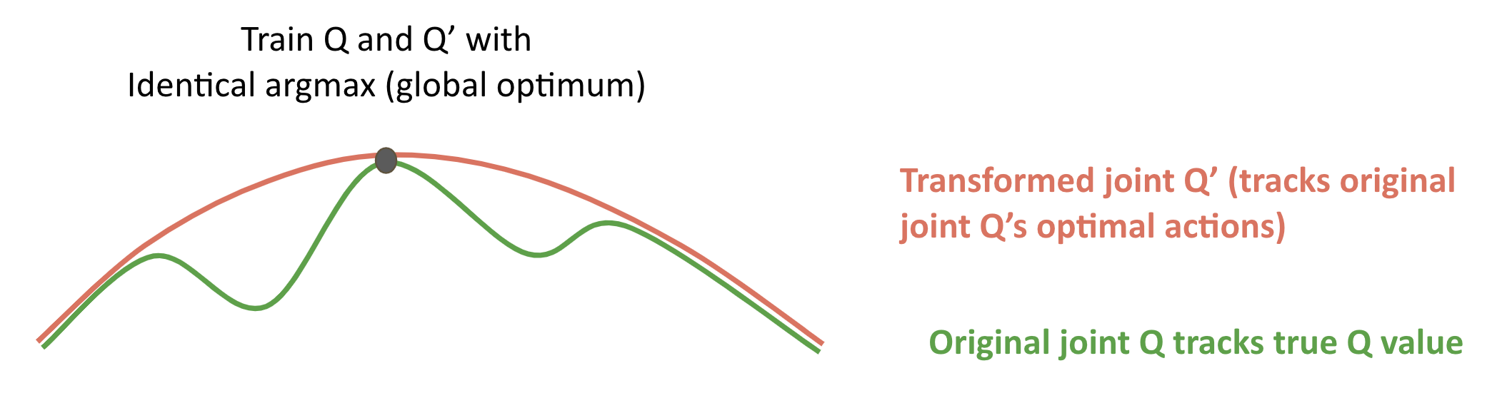
Here is a simplified visualization for intuition:

What does the architecture look like?

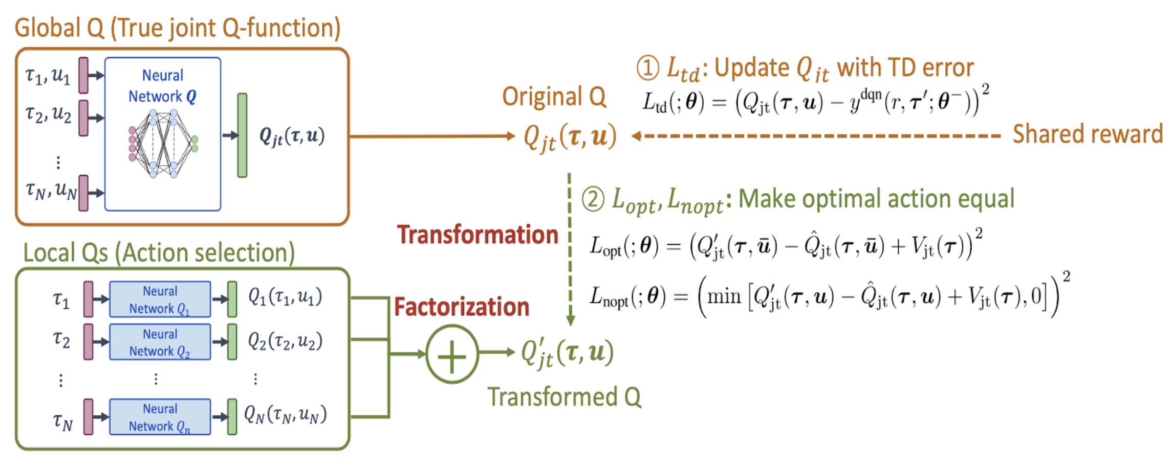
Above is a diagram of the QTran architecture from the paper. Of note, there are three neural networks, all sharing parameters:

• an individual action-value network: [Qi]
• a joint action-value network: Qjt
• a state-value network: Vjt

The first is used for decentralized execution and additively for calculating joint Q prime. The second is used for approximating the true joint Q value. The third is used in combination with joint Q prime to ensure factorization during learning.

How does this even work?

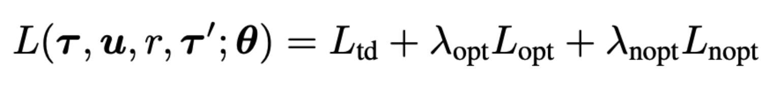
All three are neural networks, sharing parameters and an objective loss function. The loss has three components:

The first component is the temporal difference loss (TD error), which is based on a standard deep Q network. It trains the joint Q function to approximate the true joint Q function, and is an approach others have used previously with success.

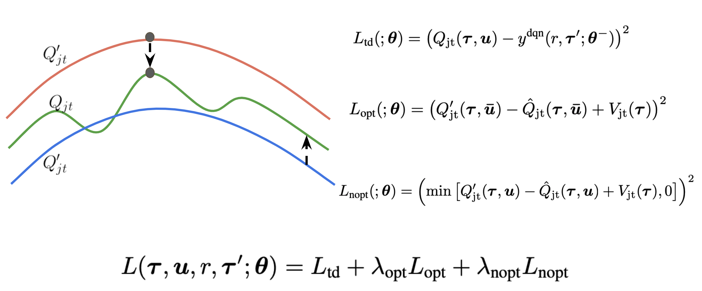
The novelty of QTran lies in the second and third components of the loss, which ensure factorizability by training joint Q prime (which is simply the sum of the individual Q functions by definition) to match the optimal actions of joint Q.

The second component (opt for optimal) adds to the loss if joint Q prime is greater than joint Q in the optimal action case. The third part of the loss adds to the loss if joint Q prime is less than joint Q in the non-optimal case. In Lopt and Lnopt, joint Q is denoted as joint Q hat because these portions of the loss are not used to train joint Q. In the author’s implementation, this is done by calling Tensorflow’s stop_gradient command on joint Q hat.

The total loss then just becomes a sum of all three components. Visually, this can be represented like this:

More

• QTran Presentation Slides
• Presentation on YouTube (a bit rough, as this was an informal run)

References

[1] Son, Kyunghwan, et al. “QTRAN: Learning to Factorize with Transformation for Cooperative Multi-Agent Reinforcement Learning.” arXiv preprint arXiv:1905.05408 (2019).

[2] Rashid, Tabish, et al. “QMIX: monotonic value function factorisation for deep multi-agent reinforcement learning.” arXiv preprint arXiv:1803.11485 (2018).